Getting Started with CountESS

CountESS is more like a toolbox than a single program: it can do all sorts of things, but that makes it a little tricky to work out how to get started. This tutorial attempts to walk you through some simplified examples to demonstrate how to solve common bioinformatics tasks with CountESS.

Demo Files

The countess-demo project provides a collection of demonstration files for use in these examples. Demo files consist of randomly generated data. Any resemblance to organisms living or otherwise is coincidental.

You can download a ZIP of the files here. or clone the repository using:

git clone https://github.com/CountESS-Project/countess-demo/

Example 1: Reading & Counting Sequences

For this simplified example, we’ll load up two CSV files with DNA sequencing data, count the population of each variant at two time points and score the variants using the ratio of their counts.

Load this example up with countess_gui example_1.ini.

There are five nodes in this CountESS pipeline, each of which transforms the data and then passes it to the next node. CountESS can also perform operations in parallel, but for the moment we can understand each of these steps as happening sequentially.

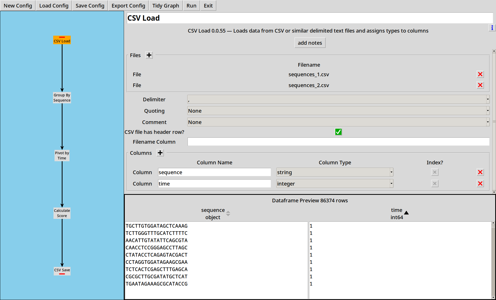
1. Loading CSV files

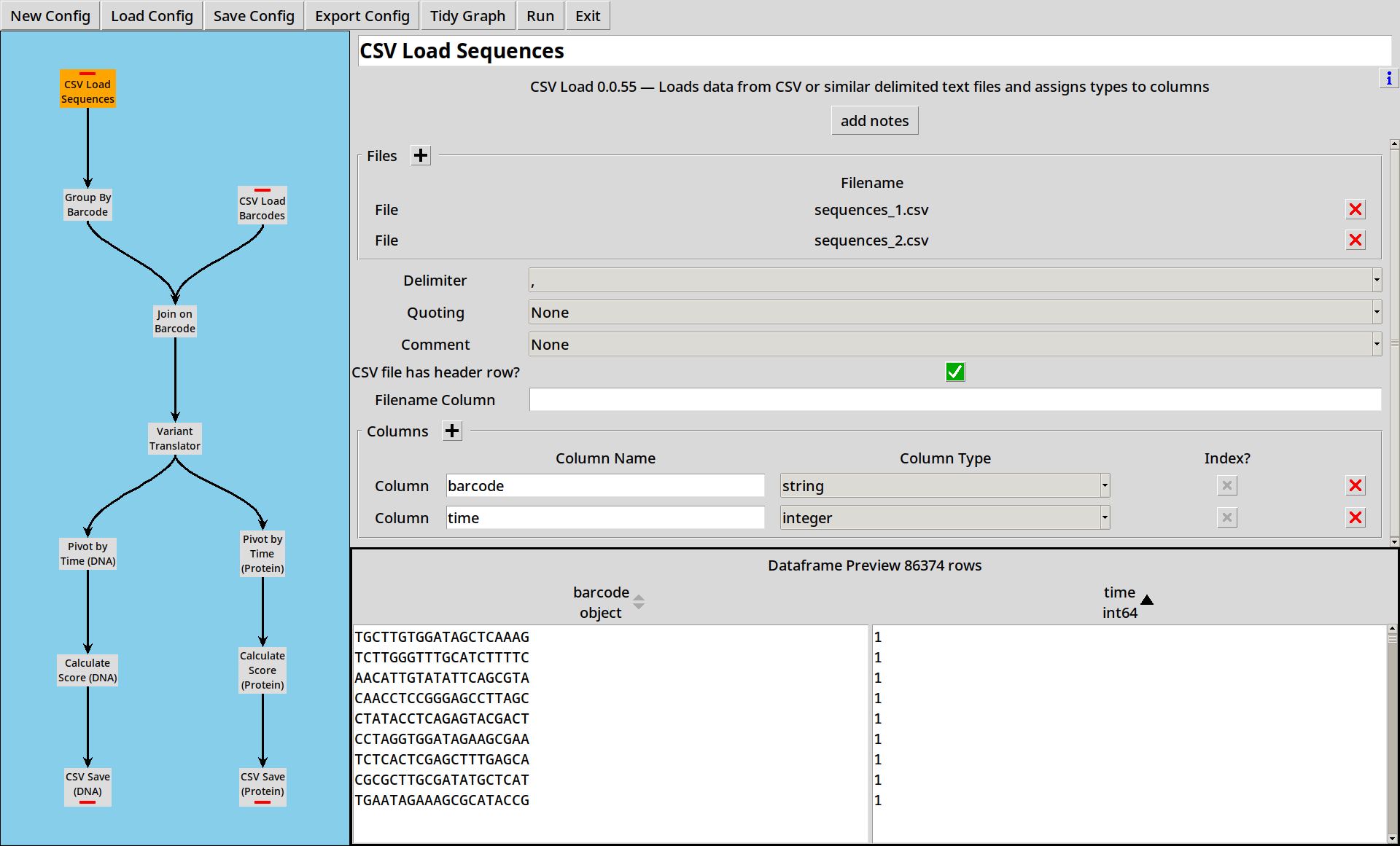
Sequences are in the files sequences_1.csv and sequences_2.csv which just contain a sequence column with raw DNA sequences and a time column.

sequence,time
AGTTCGAGGACATGGTGAGT,1
GATGTCCTAAGGGTCGATTC,1
TTCAGTACCTAAACTATGTT,1
TTTATATTTCGAGTGAATGT,1
CAACGAGAGATGTAGGAGAA,1
GTAACAGGAGTCATGTTTCC,1

(etc)

Our first step just reads these two files in.

Sequence data can also be loaded from other file formats such as FASTQ, see Example 3
CountESS can also read Gzipped CSV and FASTQ files, and this can be faster to read than plain files, depending on your platform.
With larger files, reads are limited to 100,000 rows when previewing.

2. Grouping by Sequence

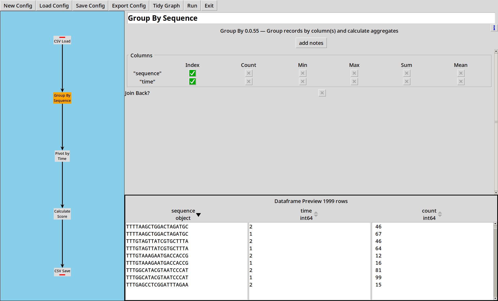
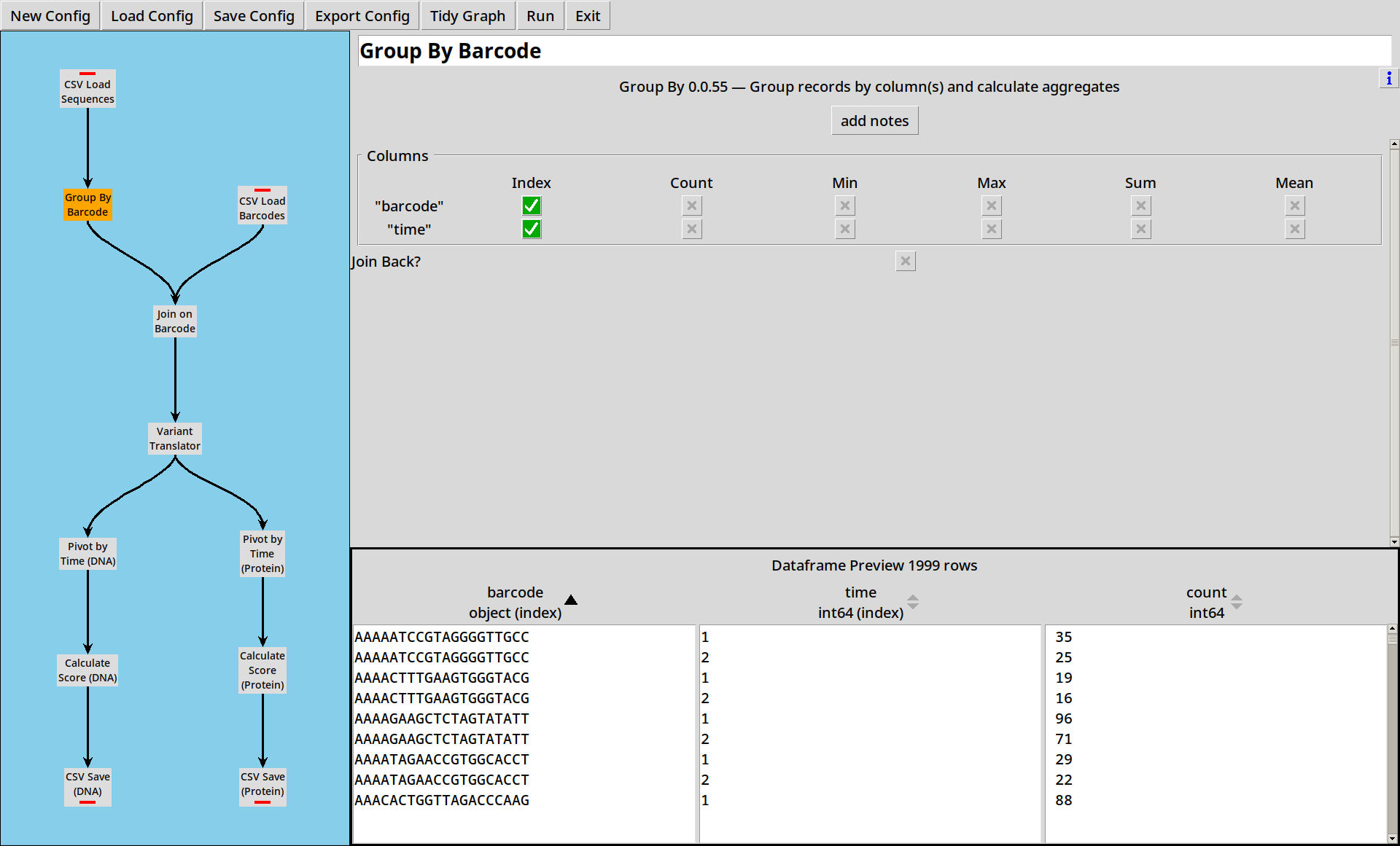
We now have a dataframe with all our raw sequences in it. Next we want to count how many times each sequence appears at each time point.

The Group By tool lets us specify some columns to index by. If no other operations are selected, it will count the number of rows corresponding to each index value, and put this into a column called “count”.

The preview pane can be sorted by columns to get a better understanding of your data.
The “count” operation will count how many rows belong in the group. If your data already has “counts”, select “sum” on that column to sum the counts for each group.

3. Pivoting by Time

We’ve now got separate counts for each sequence at each time point, but we want to compare counts for each sequence across the time points.

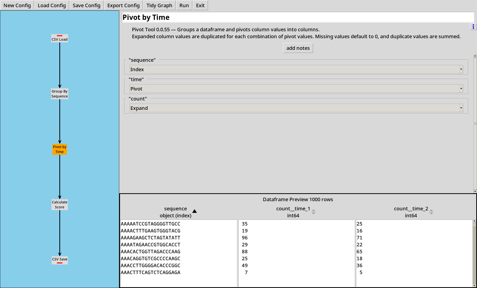
To do this, we use the Pivot Tool:

The distinct values of the “Pivot” column(s) are used to expand the data in the “Expand” column(s) into new columns.

In this case, we’re expanding the column count into two new columns, count__time_1 and count__time_2.

If there are duplicate values in the index, the expanded numbers get summed.
If there are missing values, they default to zero.
CountESS only supports pivoting up to 200 output columns.

4. Calculating Scores

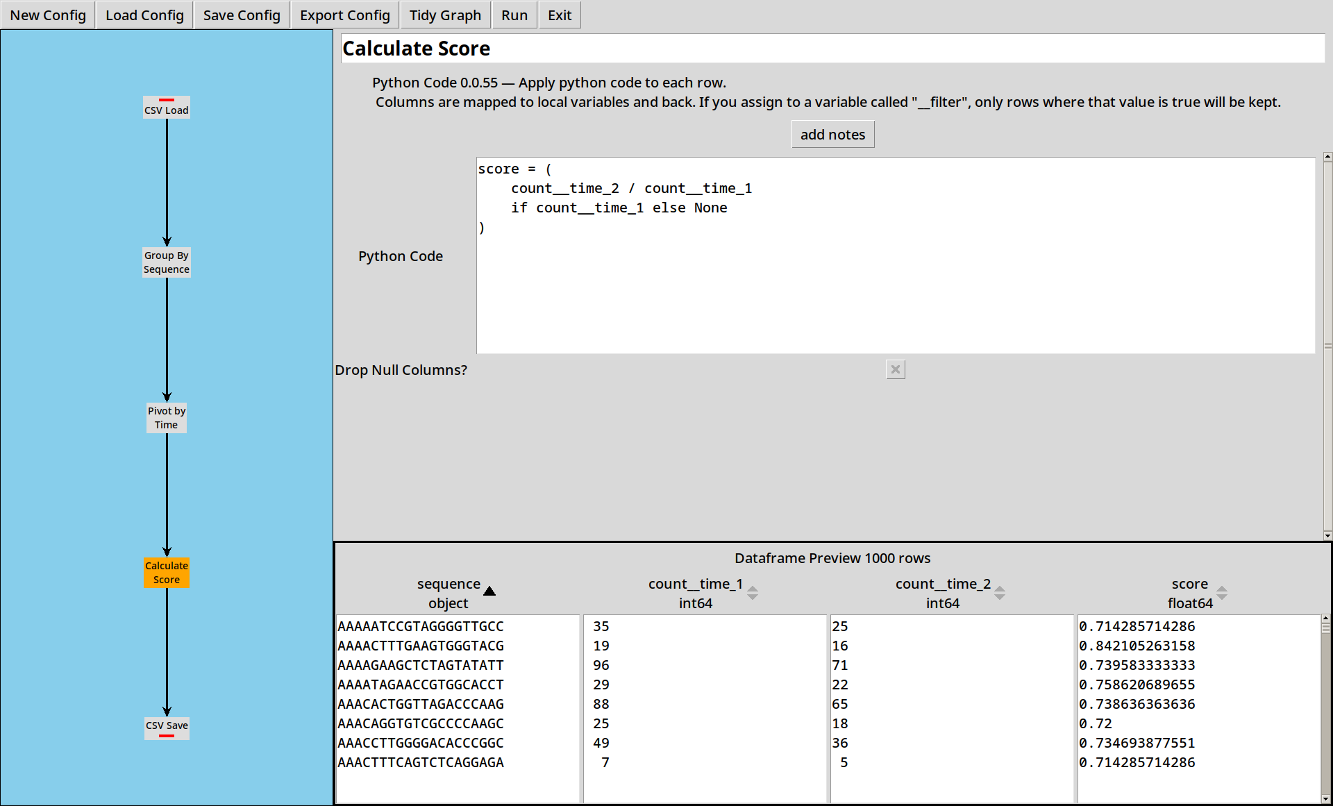
Now we have pivoted the data, for each sequence we have counts at two different time points. We want to calculate scores from the counts by dividing one by the other:

The Python Code tool lets us write small expressions in Python and apply them to each row of the table. In this case we’re calculating a simplified score as the fraction of sequences which have survived from time 1 to time 2.

5. Saving Results

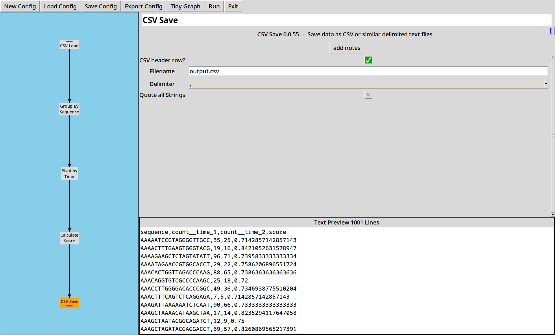
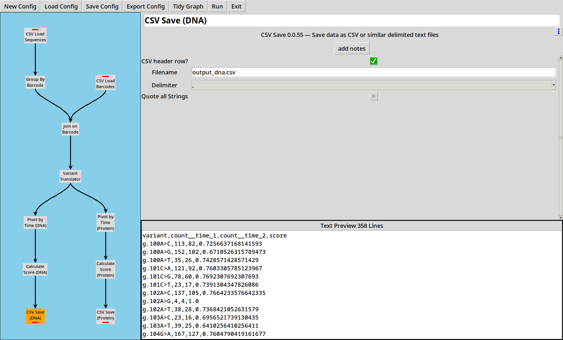
Now we have a score for each sequence, we need to write our data out somewhere. The CSV Save tool lets us save our output in a CSV file for easy use elsewhere.

The output ends up looking like:

sequence,count__time_1,count__time_2,score
AAAAATCCGTAGGGGTTGCC,35,25,0.7142857142857143
AAAACTTTGAAGTGGGTACG,19,16,0.8421052631578947
AAAAGAAGCTCTAGTATATT,96,71,0.7395833333333334
AAAATAGAACCGTGGCACCT,29,22,0.7586206896551724
AAACACTGGTTAGACCCAAG,88,65,0.7386363636363636

(etc)

The “Text Preview” is just that, a preview. Nothing is written to the file until you click “Run”.

Example 2: Translating Barcodes & Calling Variants

Load this example with countess_gui example_2.ini.

Translating Barcodes

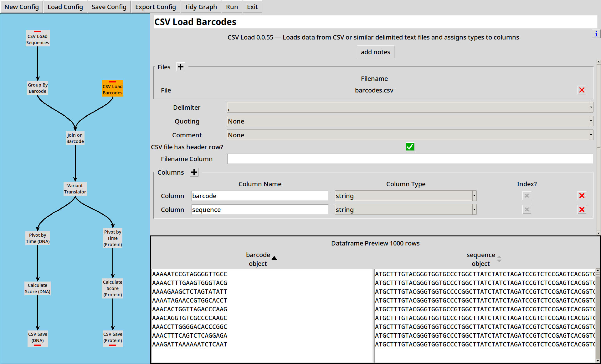
Often, rather than direct sequencing, our sequencing files are full of “barcodes”, and we need to use a barcode map to translate to an actual sequence.

In this example, we’re working with a simple barcode map barcodes.csv, each row of which translates our random 20 base barcodes to various SNVs of a 147-base protein coding sequence.

barcode,sequence
ATTCCCGTAATCTACGATTA,ATGCTTTGTACGGGTGGTGCCCTGGCTTATCTATCTAGATCCGTCTCCGAGTCACGGTCGAATTTAGGTACTGCACTATCCTTTGAGGCGGGAAGGGCCACAAGGGCCGACCCTTGTCGGATAAAATTTGCTAAGAGGAAGGTCTAG
AGTCACAACCAAACCATGGA,ATGCTTTGTACGGGTGGTGCCCTGGCTTATCTATCTAGATCCGTCTCCGAGTCACGGTCGAATTTAGGTACTGCACTATCCTTTGAGGCGGGAAGGGCCACAAGGGCCGACCCTTGTCGGATAAAATTTGCTAAGAGGAAGGTCTAG
TTACGGTCTGCGTTGGAATC,ATGCTTTGTACGGGTGGTGCCCTGGCTTATCTATCTAGATCCGTCTCCGAGTCACGGTCGAATTTAGGTACTGCACTATCCTTTGAGGCGGGAAGGGCCACAAGGGCCGACCCTTGTCGGATAAAATTTGCTAAGAGGAAGGTCTAG
AGGGCCGTGCCAAGTGCAGT,ATGCTTTGTACGGGTGGTGCCCTGGCTTATCTATCTAGATCCGTCTCCGAGTCACGGTCGAATTTAGGTACTGCACTATCCTTTGAGGCGGGAAGGACCACAAGGGCCGACCCTTGTCGGATAAAATTTGCTAAGAGGAAGGTCTAG
TGTAGTGCCGTATTTGTGGC,ATGCTTTGTACGGGTGGTGCCCTGGCTTATCTATCTAGATCCGTCTCCGAGTCACGGTCGAATTTAGGTACTGCACTATCCTTTGAGGCAGGAAGGGCCACAAGGGCCGACCCTTGTCGGATAAAATTTGCTAAGAGGAAGGTCTAG

(etc)

The first three barcodes map to the same sequence, the other two have SNVs but they are hard to spot! There are 1000 barcodes in the file, about 1/4 of which map to unmodified sequences.

First, we modify our sequence reading and grouping steps to rename the sequence column to barcode, for clarity.

Second, we add a new node to read the barcode map using the CSV Loader:

Joining

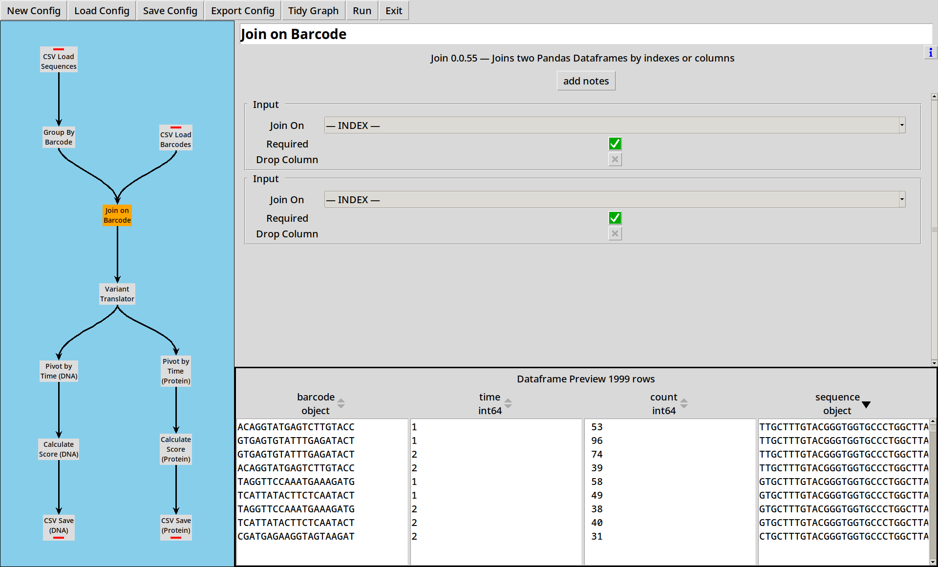
Now we add in a Join tool, which takes two inputs and joins them.

Note that while there were 1000 distinct barcodes, there are only 357 distinct sequences. Some barcodes represent duplicate variants.
By default both inputs are “required”, so this is like an inner join, but by toggling one or both flags you can perform a left, right or full join.

Calling Variants

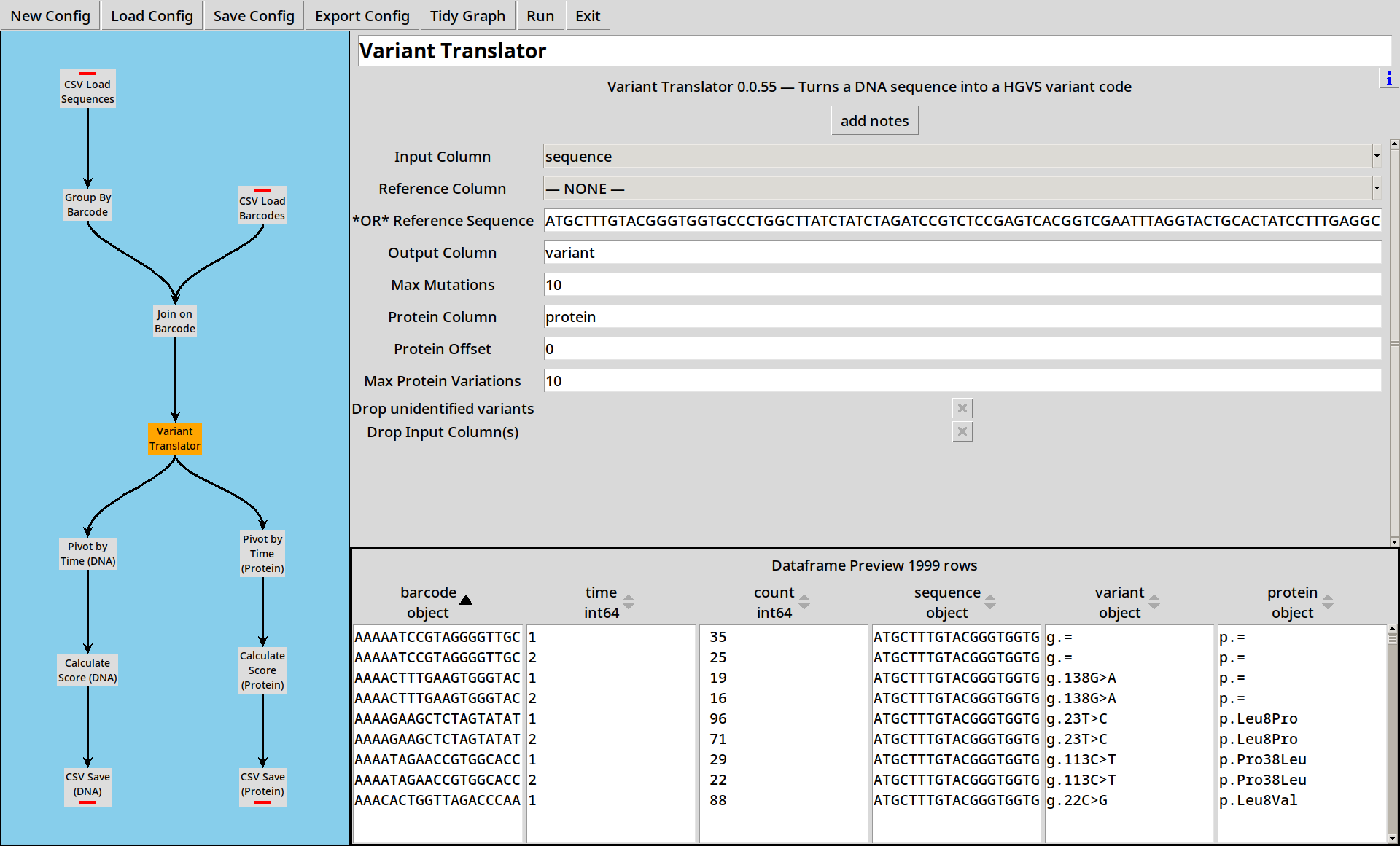
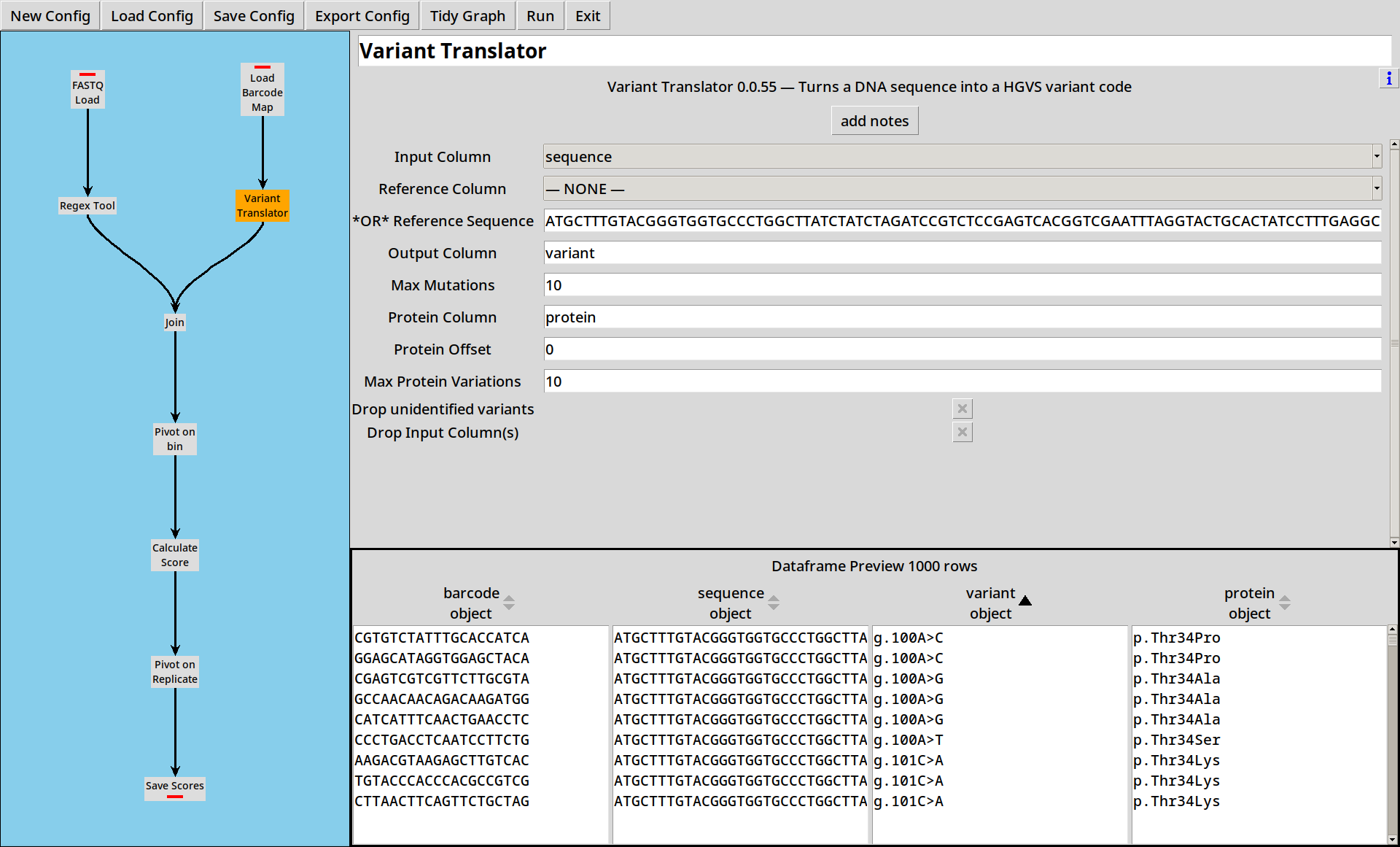
Working with long sequences is a bit unwieldy: it’d be handy to be able to process these in a more compact format. The Variant Translator plugin lets us compare a sequence to a reference sequence and extract DNA and Protein variants in HGVS format.

We add a Variant Translator to our project, and configure it with our known reference sequence:

ATGCTTTGTACGGGTGGTGCCCTGGCTTATCTATCTAGATCCGTCTCCGAGTCACGGTCGAATTTAGGTACTGCACTATCCTTTGAGGCGGGAAGGGCCACAAGGGCCGACCCTTGTCGGATAAAATTTGCTAAGAGGAAGGTCTAG

and it calculates both DNA (variant) and Protein (protein) variant strings for each sequence in the dataframe.

Quite a lot of the DNA variants turn out to be equal to the reference sequence (g.=) and even more of the Protein variants turn out to be synonymous (p.=).

Multiple Outputs

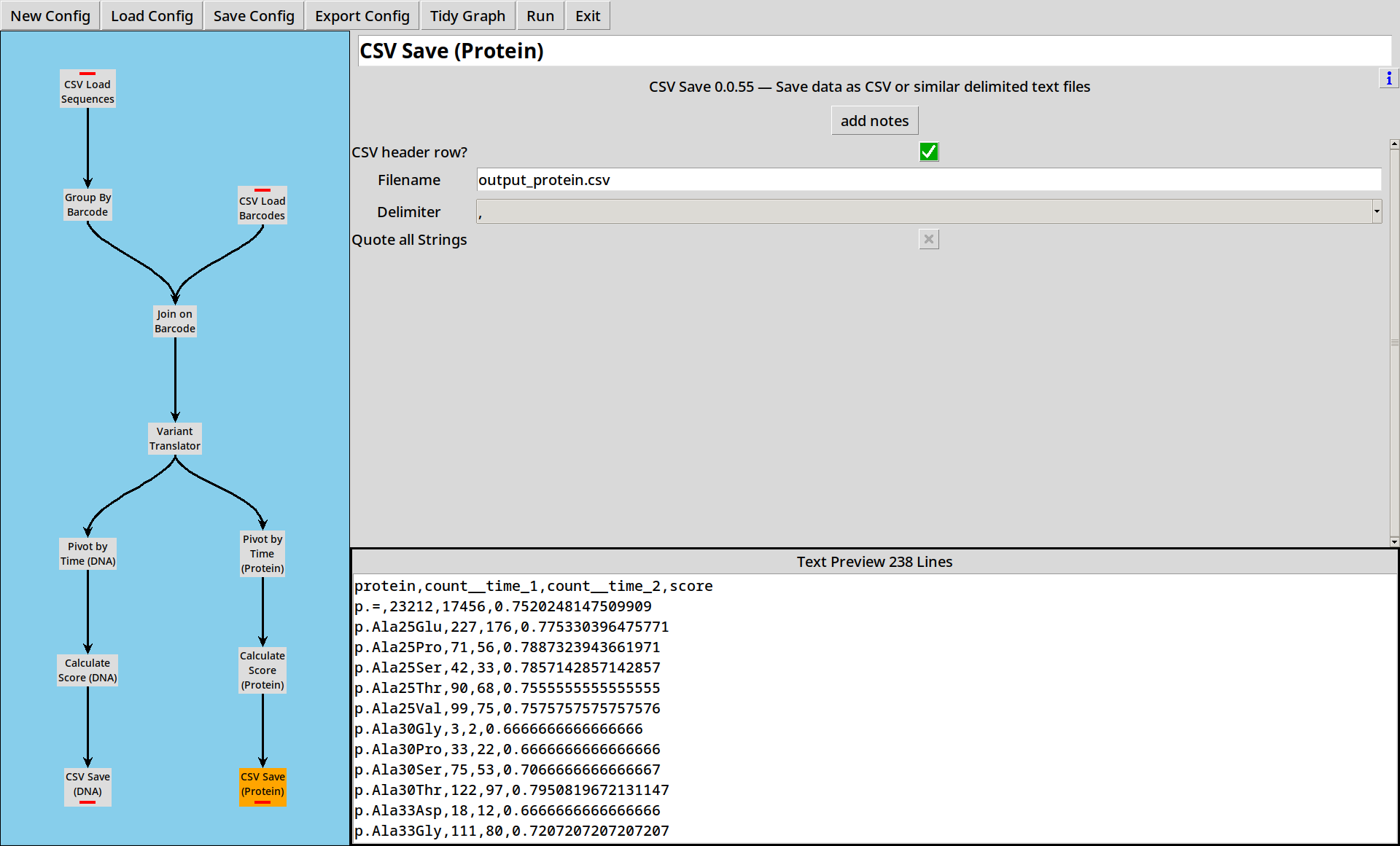
CountESS nodes can have multiple outputs. From here, we perform the same pivot, score and write to CSV steps as before, but duplicated for both DNA and Protein variants.

Example 3: FASTQ and VAMP-seq

Load this example with countess_gui example_3.ini.

Loading FASTQ

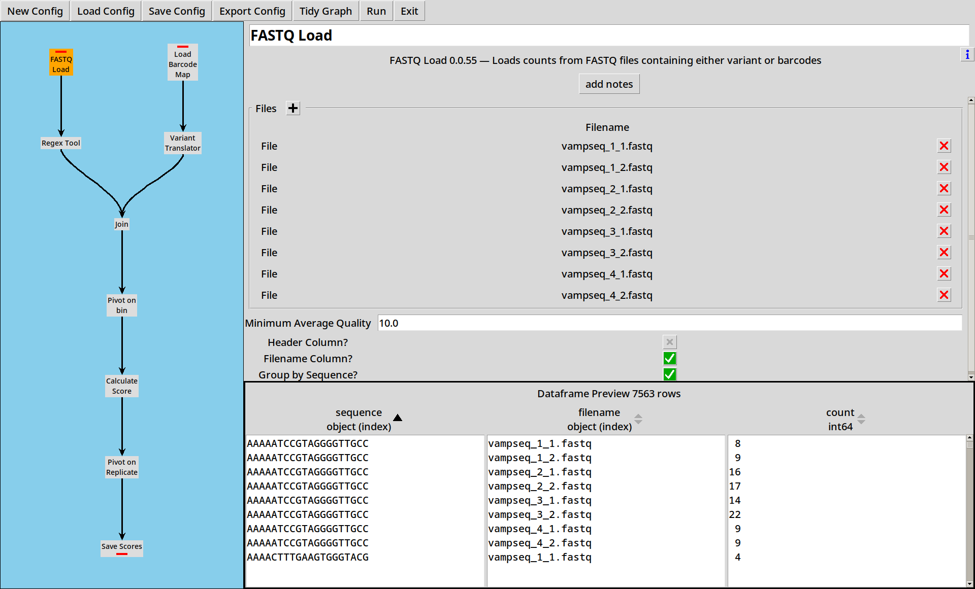
In the previous examples, we’ve loaded sequence data from CSV files, but FASTQ files are a more common format for sequence data and we can read these with the FASTQ Reader

The CSV files had a convenient time column for us to use, but our example FASTQ files do not. Fortunately, the metadata we need is available in the filename. We can select the “Filename Column?” option in the FASTQ Loader which will add an extra filename column in to the dataframe:

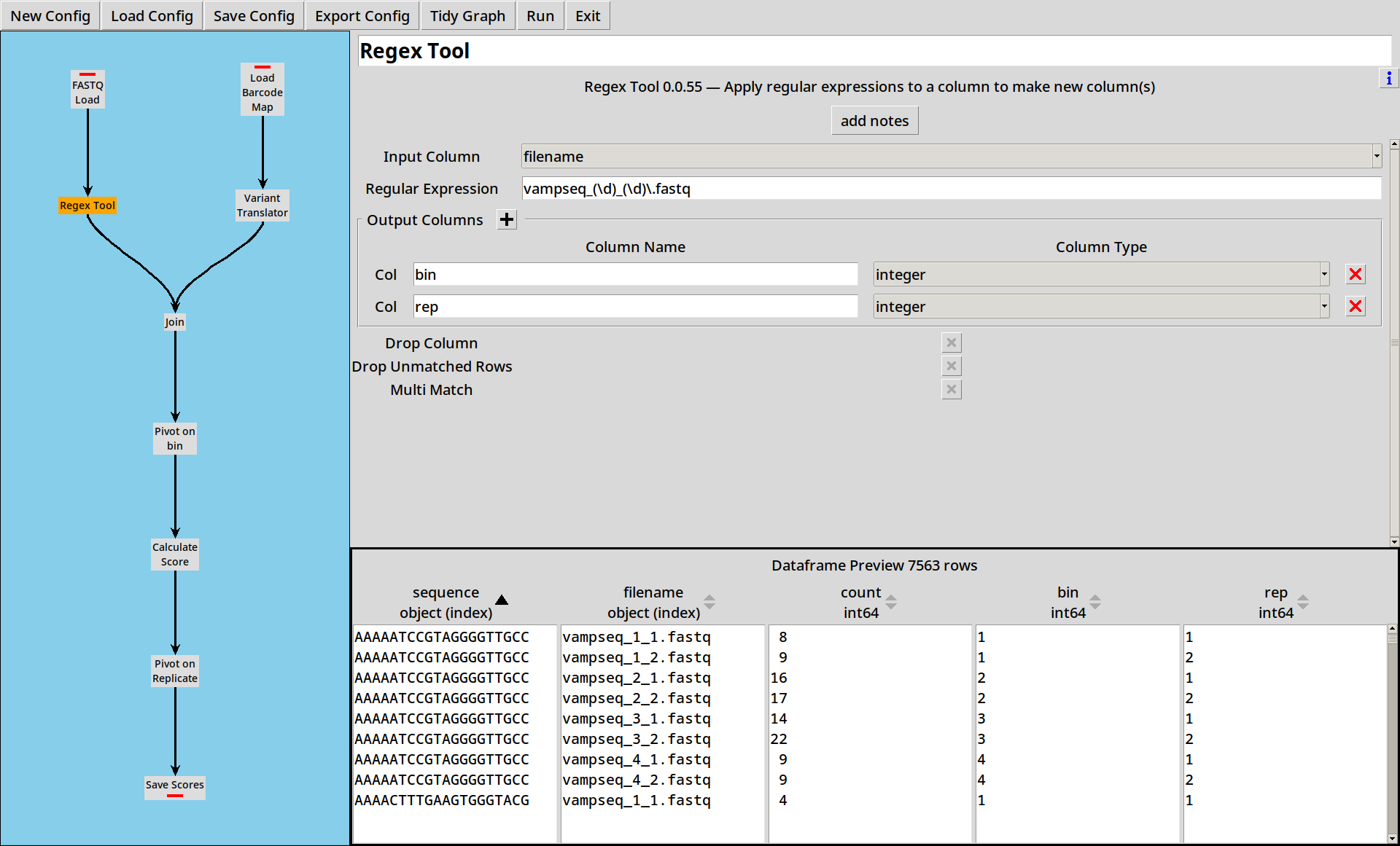
We can then use the Regex Tool to break this filename down into its useful parts, extracting bin and rep columns from the filename:

In the previous example, we chose to insert the Variant Translator after the Join for clarity, but when we have many more sequences to call it is more efficient to call the variant once for each barcode rather than once for each sequence:

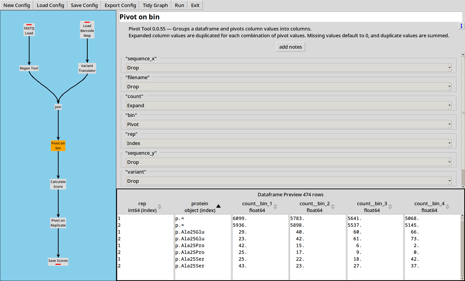
The two data sources are joined as before. We can then pivot on bin, giving us columns count__bin_1, count__bin_2, count__bin_3 and count__bin_4:

VAMP-seq

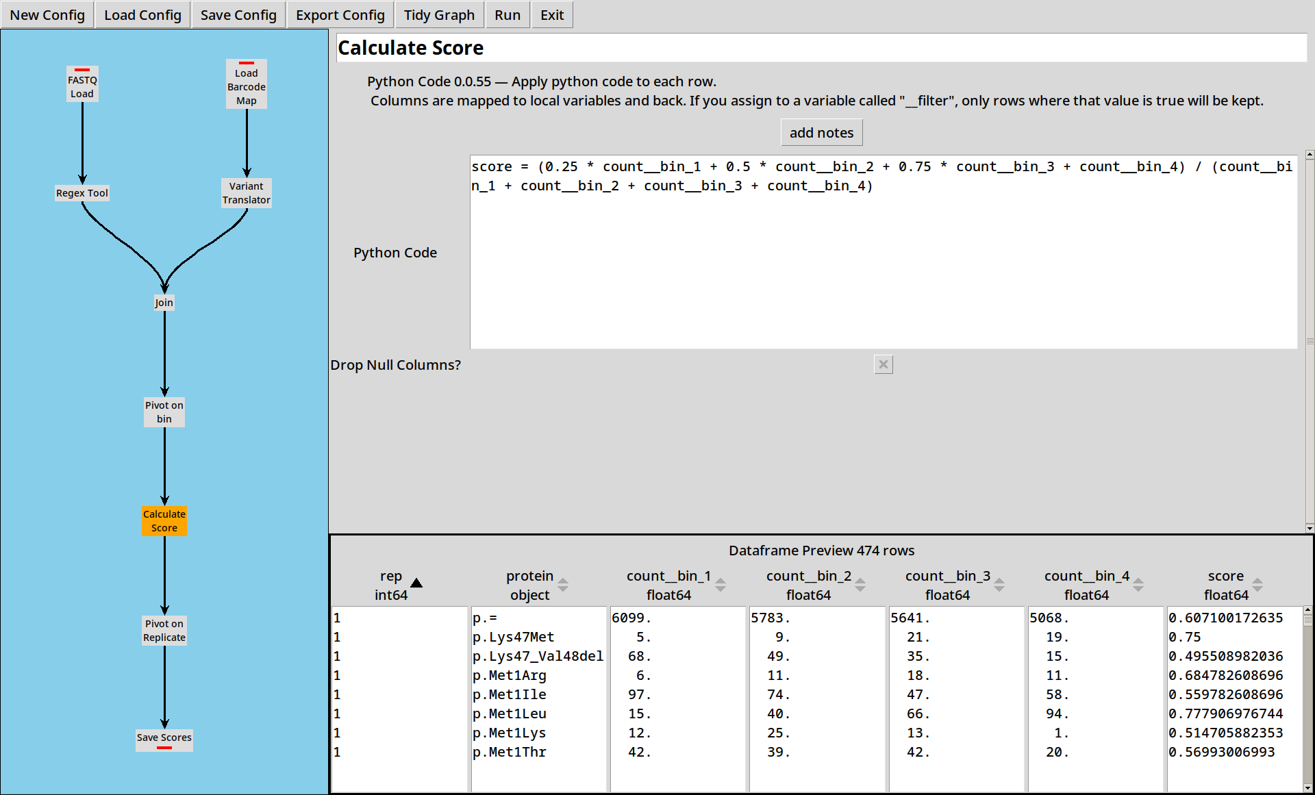
VAMP-seq uses a weighted sum of the bins to calculate a score for each variant, which is easily implemented in Python Code:

Files are then written out as before.

Example 4: External Metadata

Load this example with countess_gui example_4.ini.

The metadata you need isn’t always present in the data files or their filenames: for example your files may just be named after the order they were sequenced, or if you’ve obtained a dataset from NCBI SRA you might have just a bunch of files called SRR*.fastq.gz and an SraRunTable.txt which provides all the metadata.

In this example our data files are named data12345.fastq and so on, and we have a metadata.tsv file which maps the filenames to replicate number and a time:

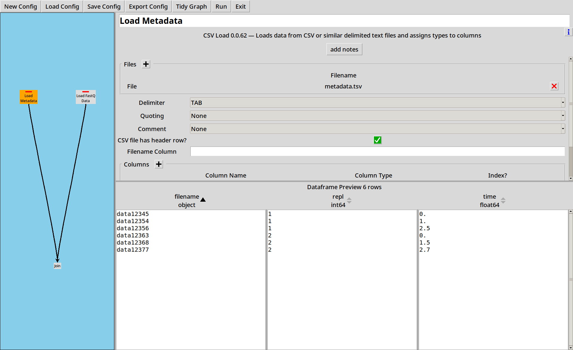
filename	repl	time
data12345	1	0
data12354	1	1
data12356	1	2.5
data12363	2	0
data12368	2	1.5
data12377	2	2.7

First we load up the metadata file, splitting the columns using “TAB” characters:

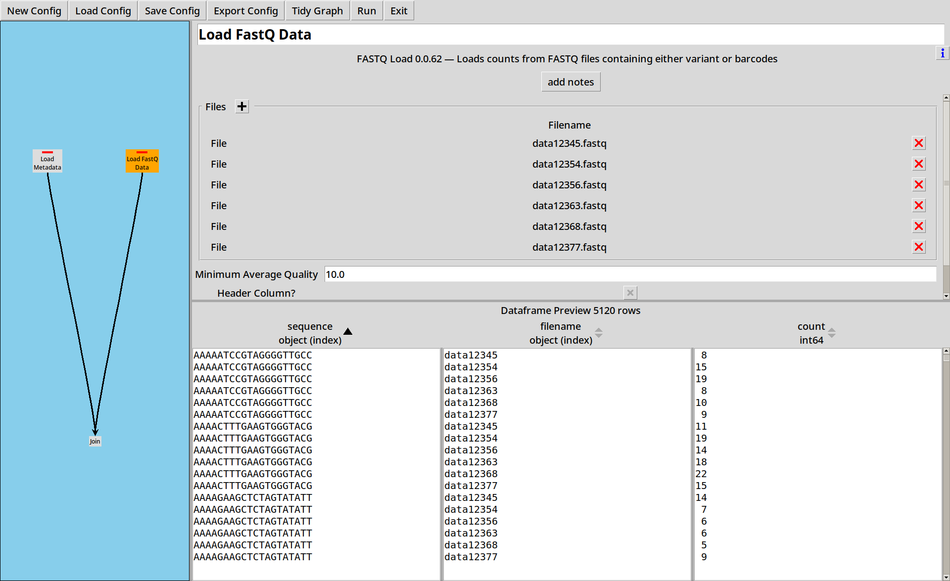
Then we load up the six data files, remembering to select the “Filename Column?” option to get the filename as a column:

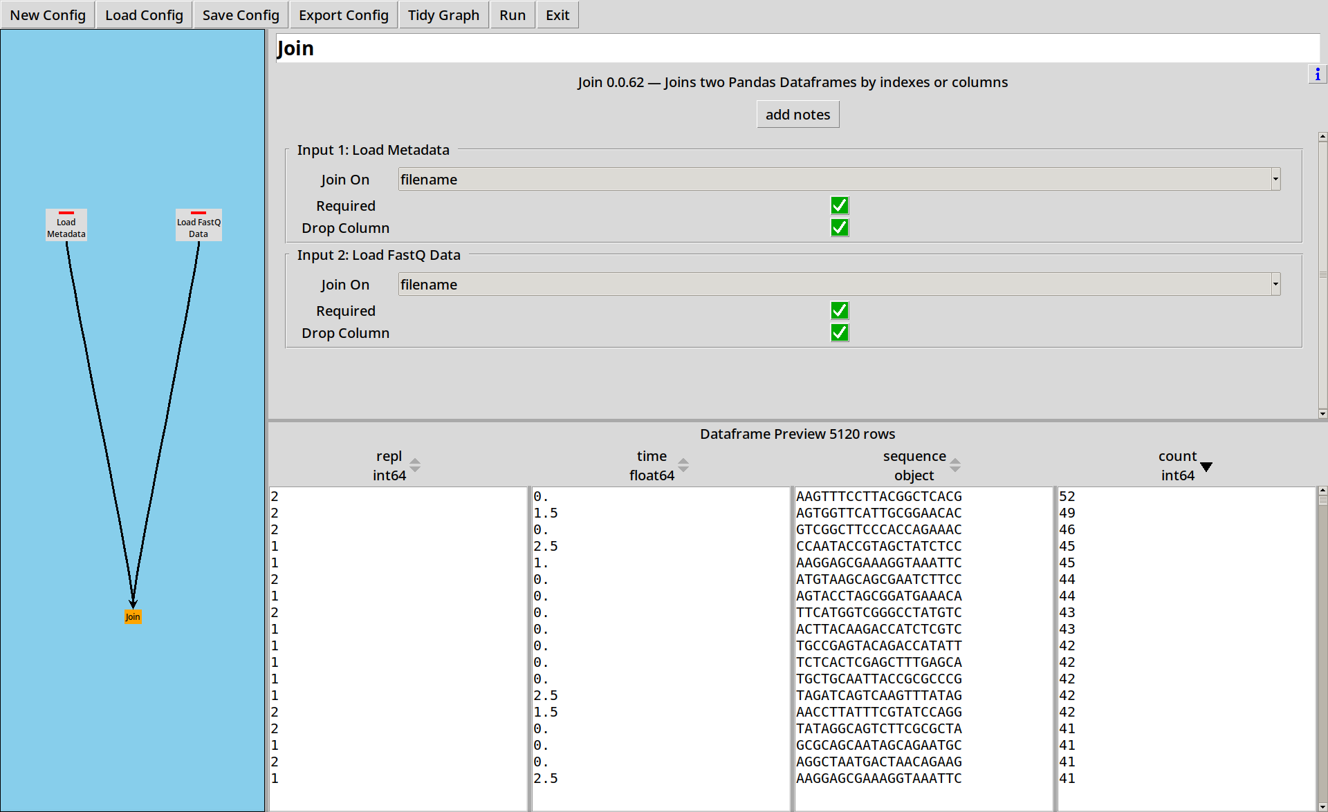
Then we can join the two together using the filename column in each: