Further Examples

Continuing on from the examples in Getting Started with CountESS let’s look at some more realistic experiments:

Example 5: Deep Mutational Scan of BRCA1

This example is based on a small subset of a real deep mutational scan of BRCA1, testing for E3 ubiquitin ligase activity (Starita et al. 2015).

The data is taken from the Enrich2-Example project to make it easy to compare CountESS to Enrich2.

Load the example by running countess_gui example_5.ini. Note that this data set is bigger than the default limit of rows loaded in the GUI, so only a subset of the data is used until you click ‘Run’.

This is example is quite complex so let’s walk through it one step at a time:

Loading Files

The first thing to do is to load the data files.

Barcode Map

The barcode map is a simple .CSV file so we load that with the CSV loader:

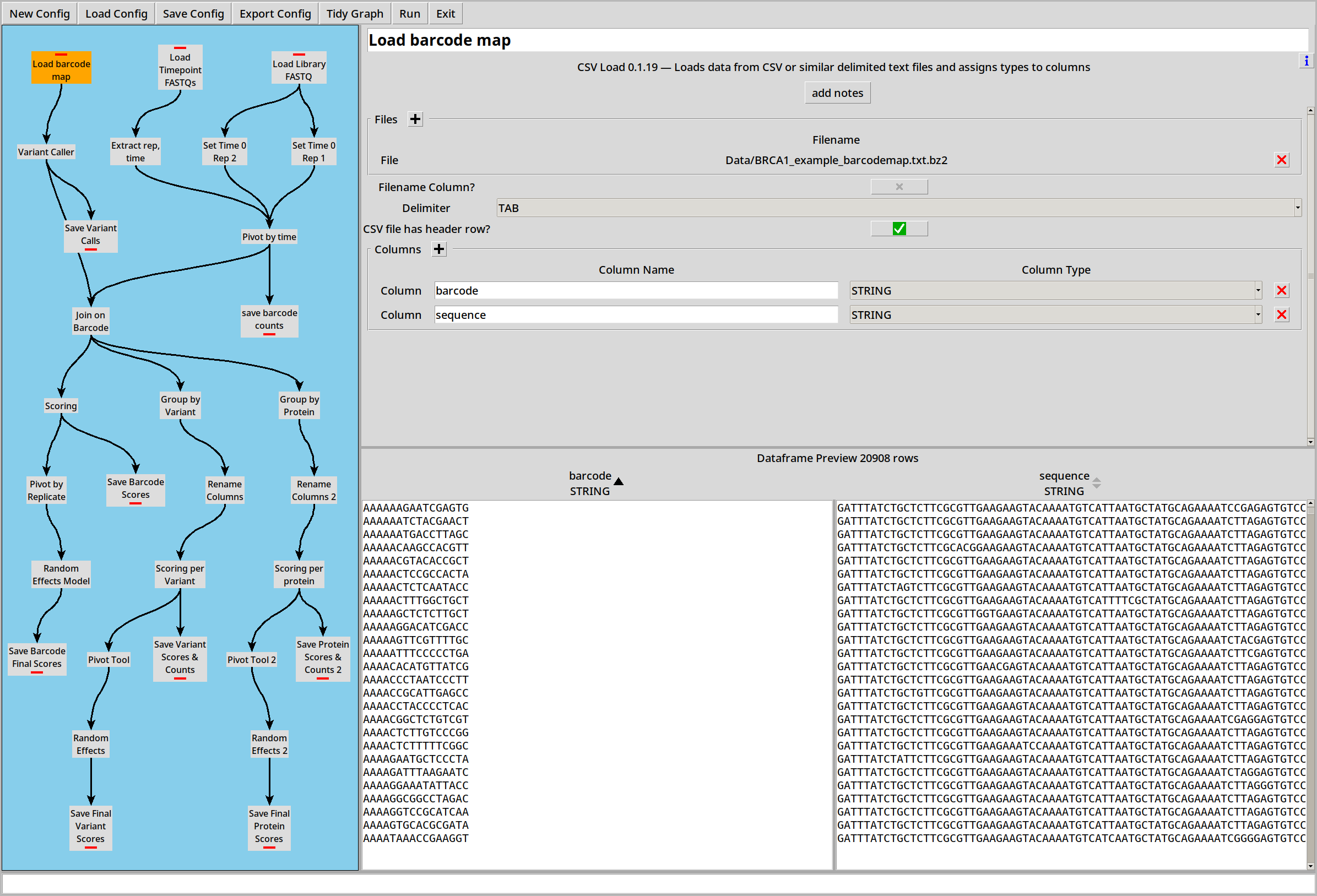
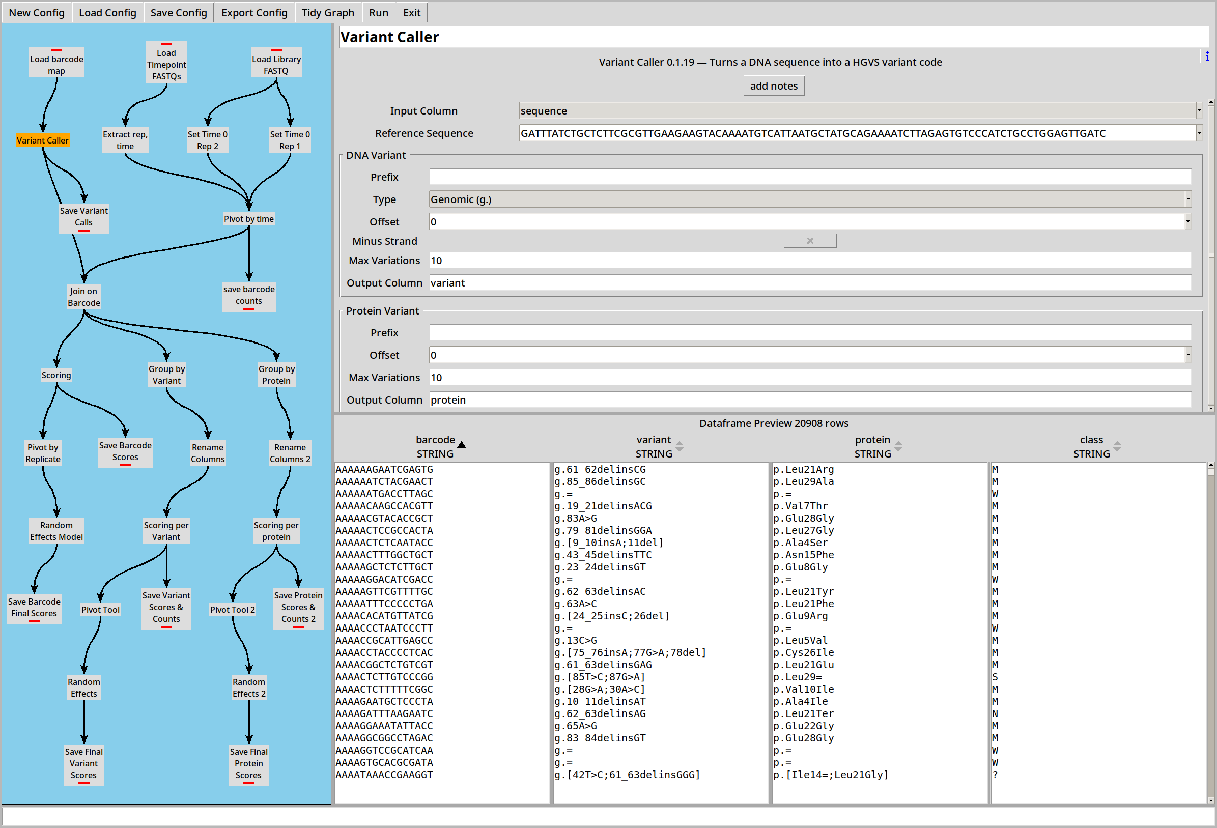
We then feed the ‘sequence’ column to the variant caller to translate the raw sequences into HGVS strings:

Replicates

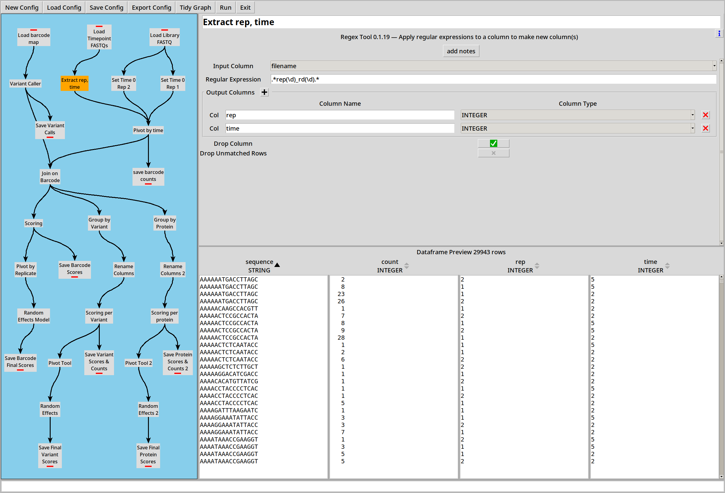
There are also four .FASTQ files representing two replicates at two time points. The replicate number and time point are encoded in the filename, so we enable the ‘Filename Column?’ option to capture this data:

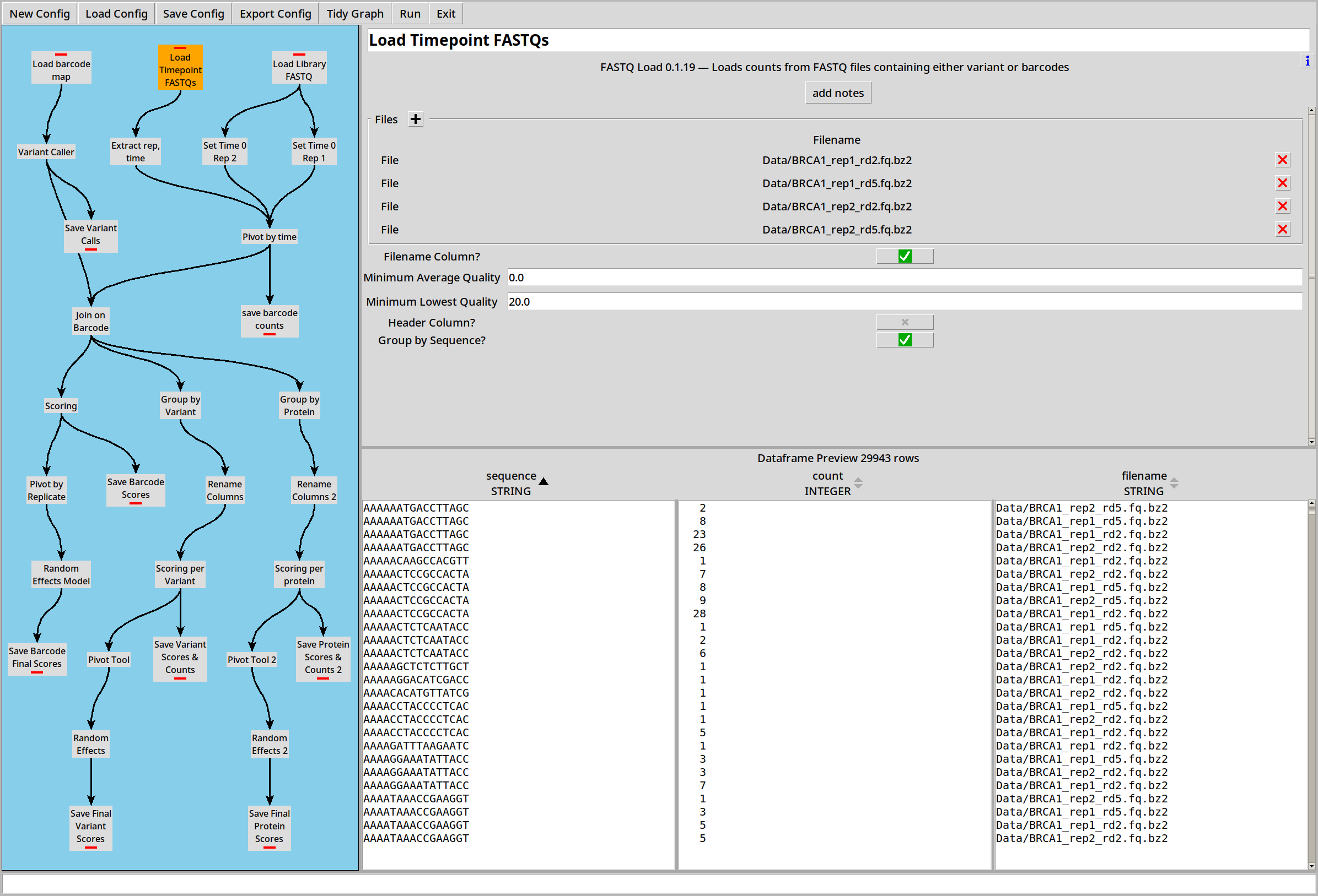
… and then the Regex plugin can split these out into separate columns called ‘rep’ and ‘time’.

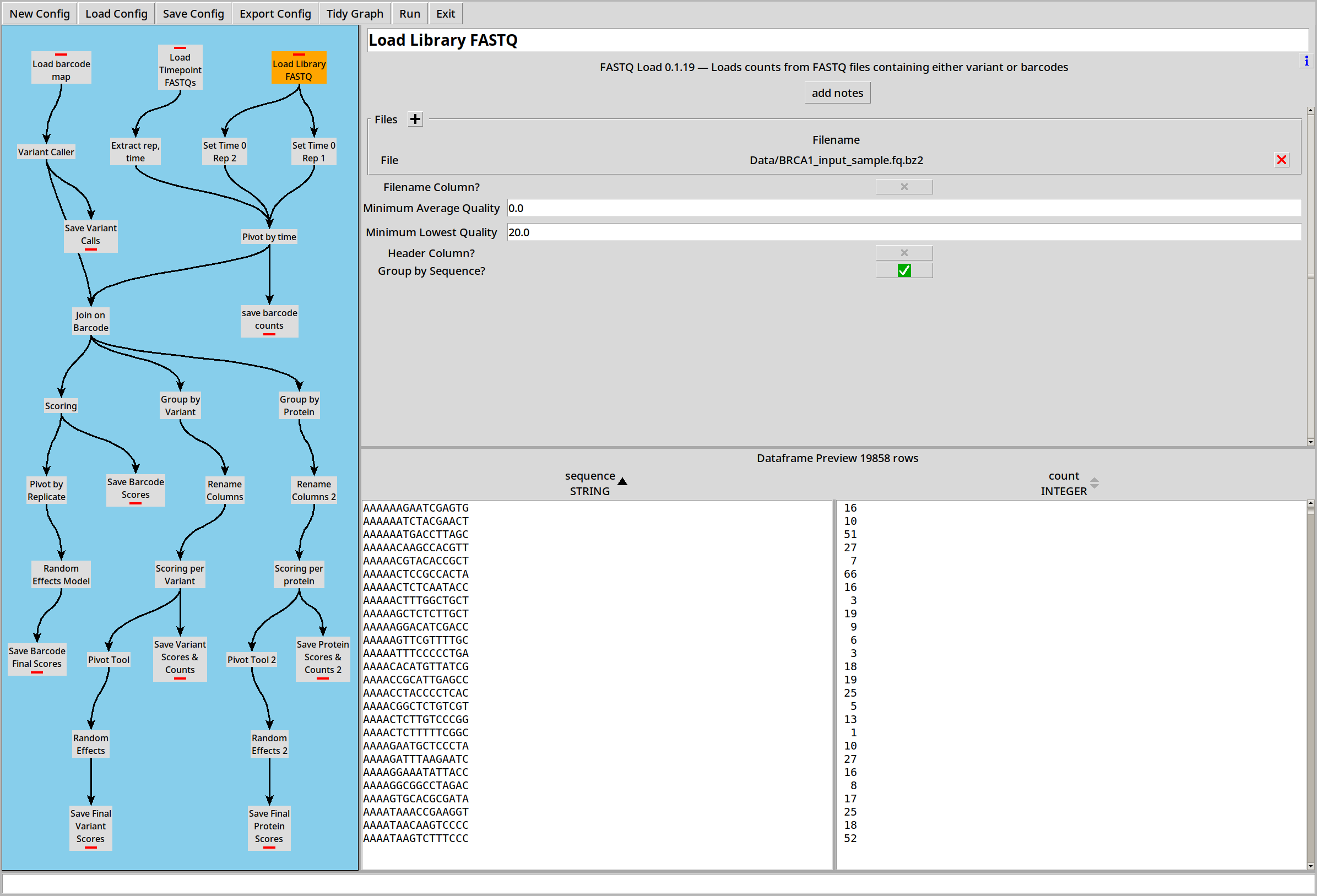
Library

There’s a single .FASTQ representing a library shared between the replicates:

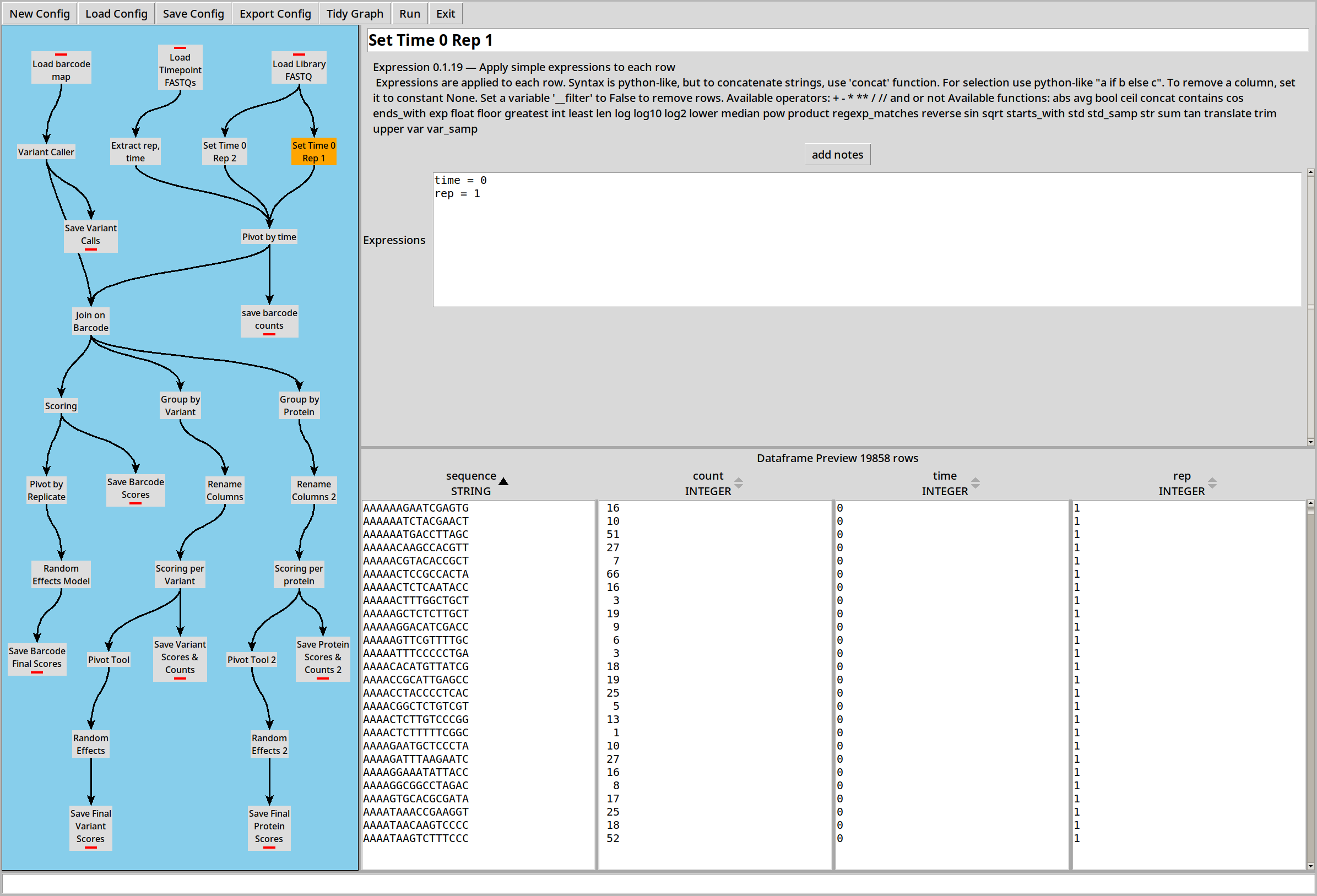
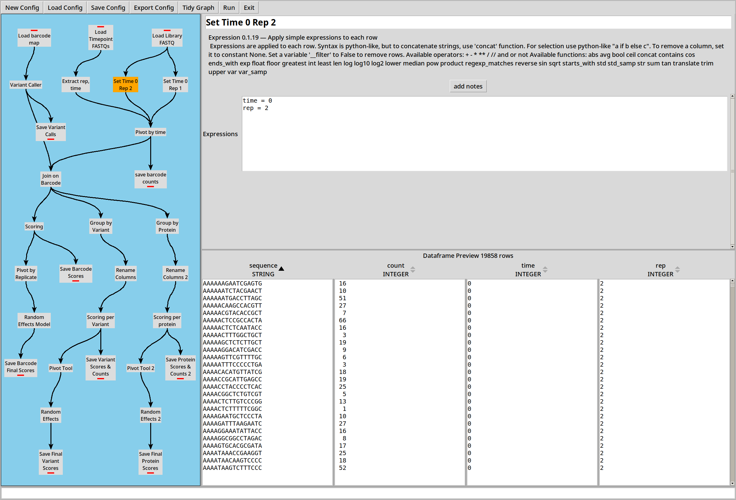
Because this library file is part of two replicates, we use two Expression plugins to make a copy of the library for each replicate, both at time 0:

Pivoting and Joining

Now we have all our data loaded, we need to pivot it and join it to bring it into a more useful form.

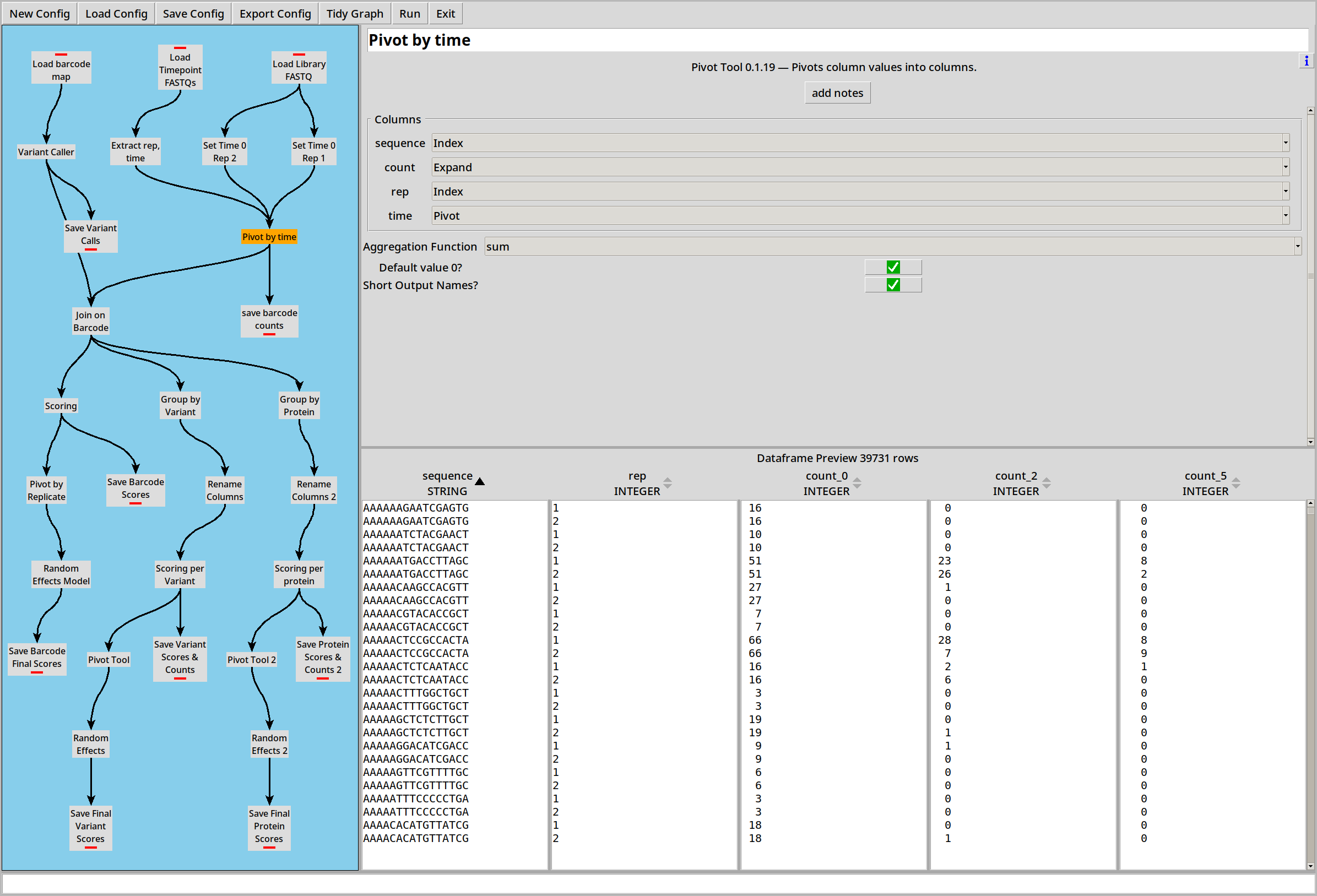
First we combine the four replicate files and the two copies of the library into a single table, and pivot it by time so that for each replicate, each row relates a barcode to three counts:

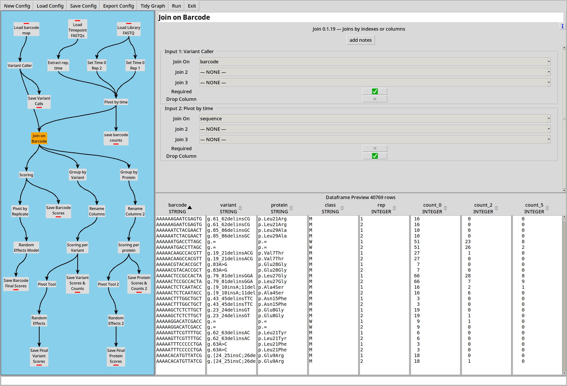
Then we can join that to the barcode map:

Scoring by Barcode

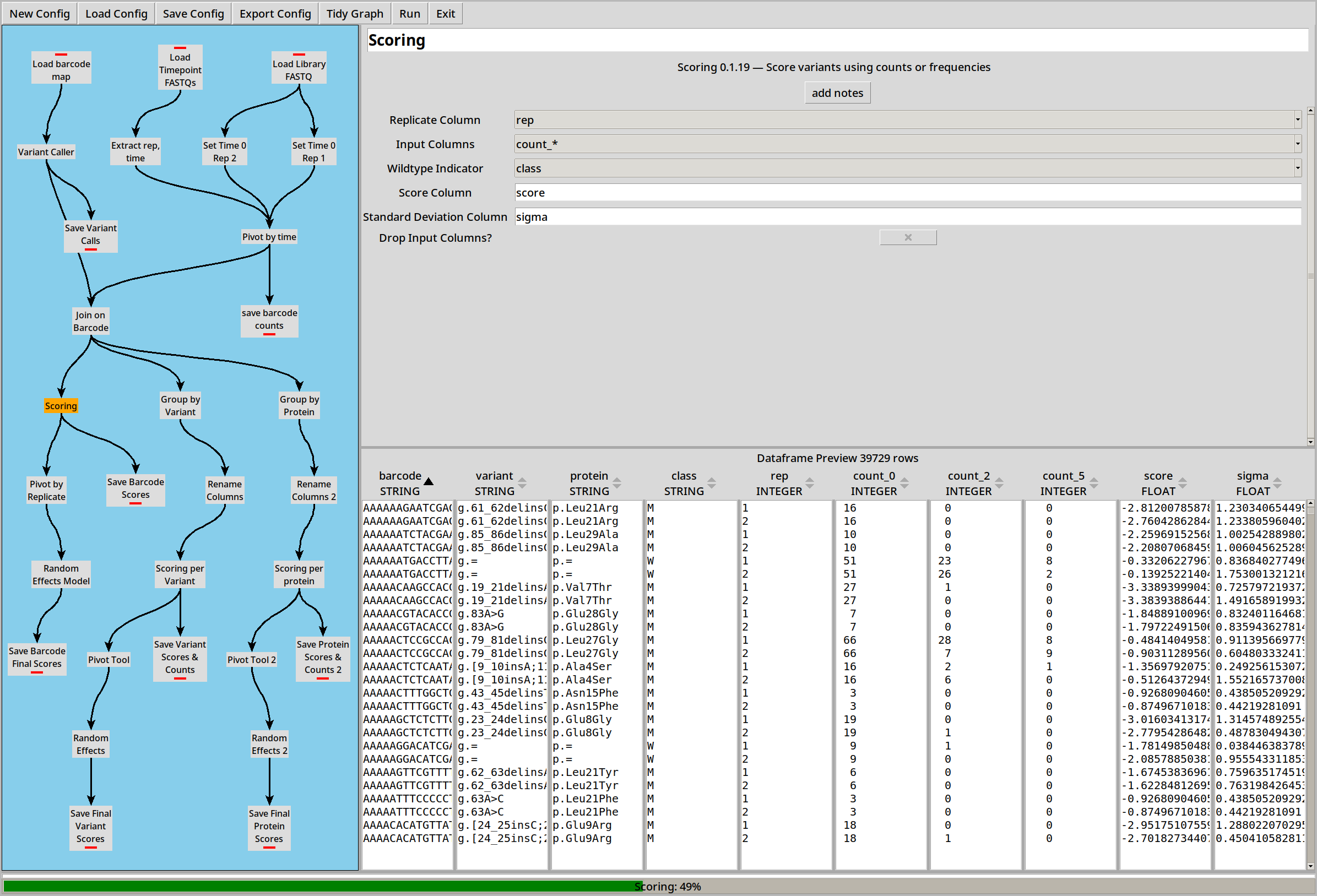
We can calculate a score for each barcode using the Score plugin. This is done using the same least-squares regression model as Enrich2:

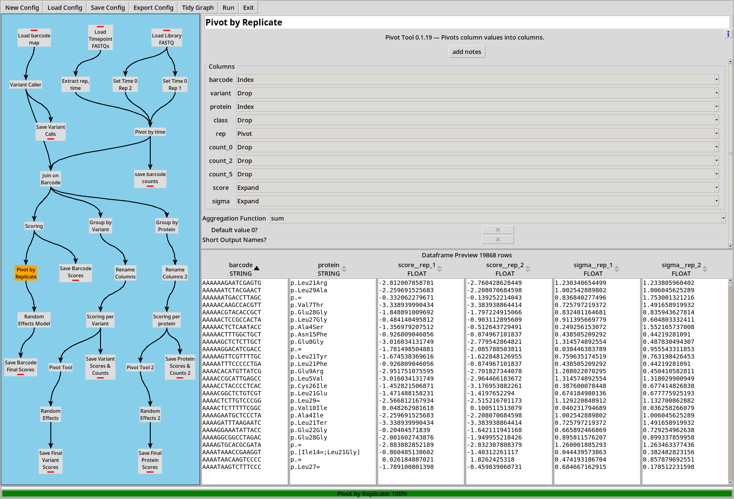
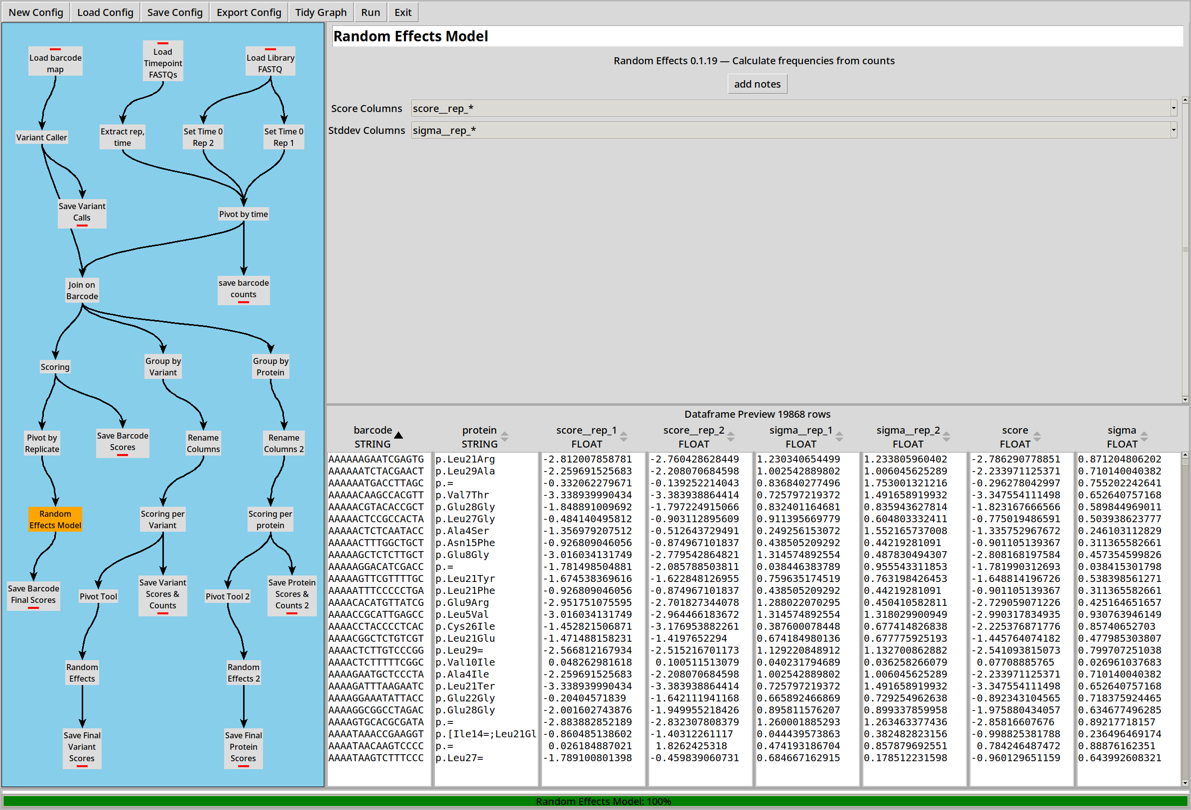
Each barcode now has a score and sigma (standard error) for each replicate. We can combine those scores into a final score by pivoting and then using a Random Effects Model to combine the individual scores and sigmas into a combined version:

Scoring by Variant

We can also choose to collate by DNA variant before calculating scores as above:

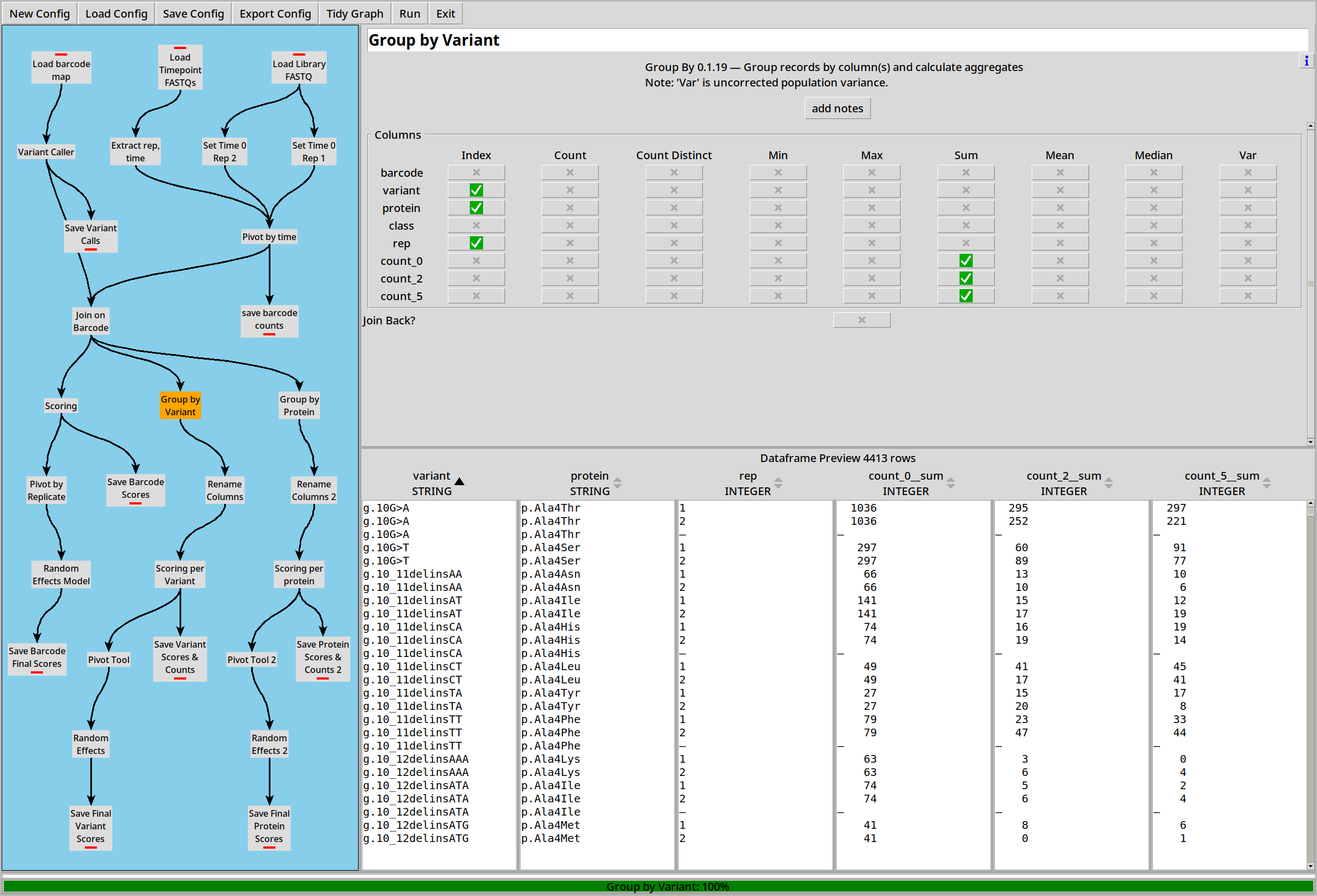
This will let us calculate scores and sigmas per DNA variant instead of per barcode:

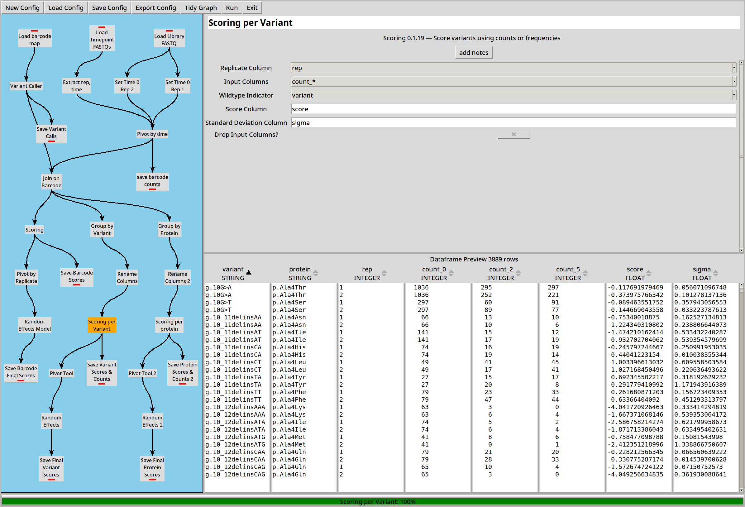
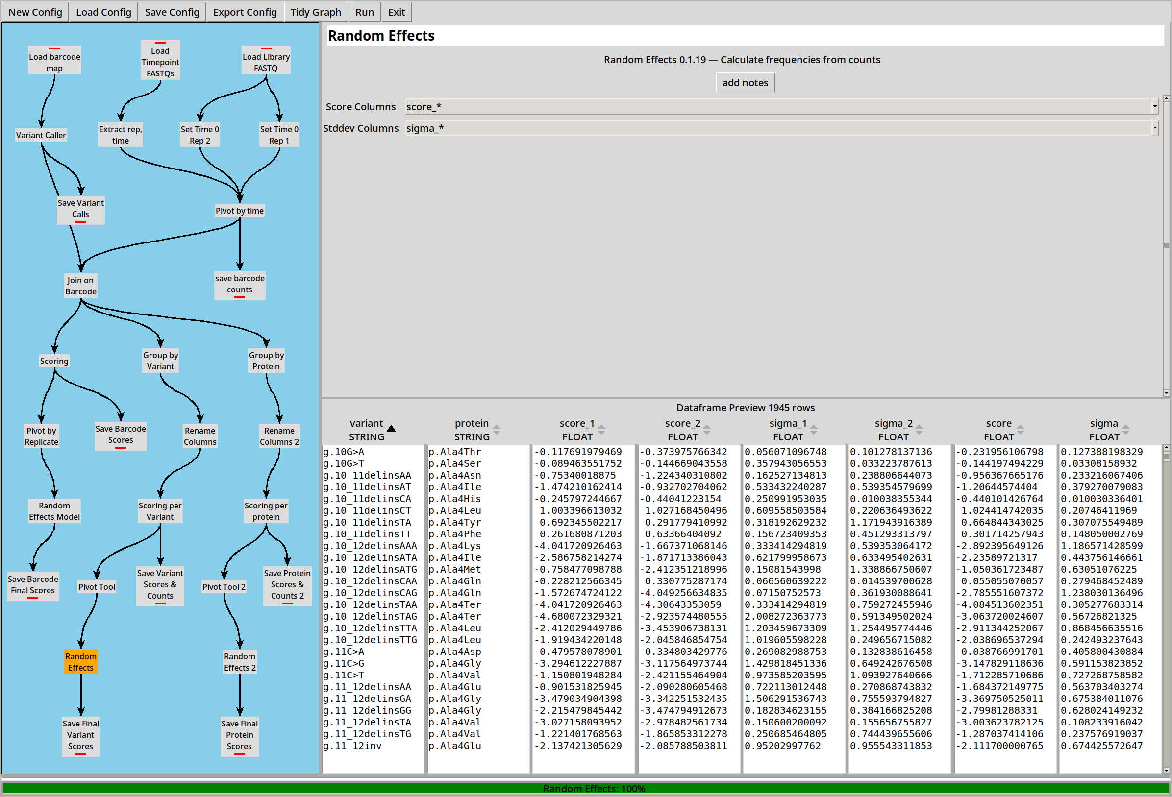
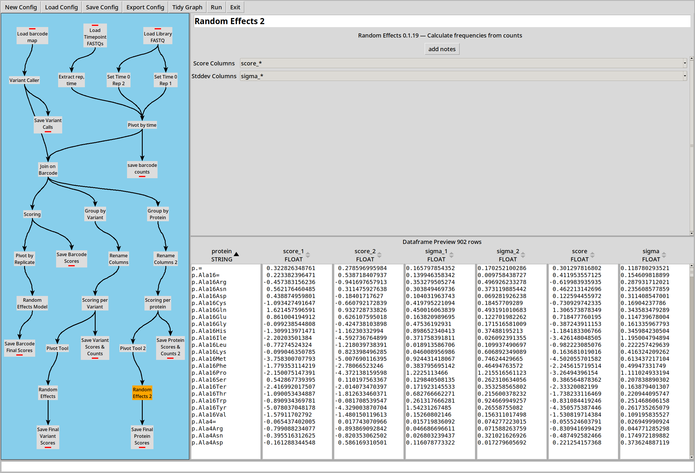
Scores can then be combined just like the “per barcode” example:

Scoring by Protein

… Or we can collate by protein variant:

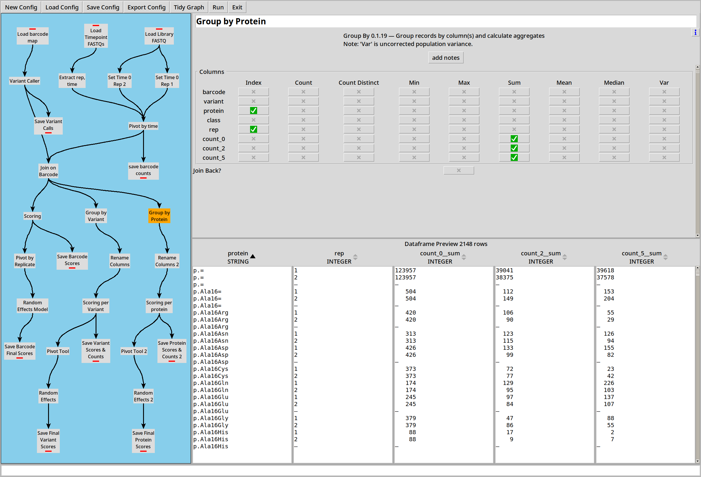
Other Options

The above example uses two replicates and three time points. If only two timepoints are available, the scoring plugin falls back on the “log ratio” version of the scoring formula, also as per Enrich2.

If there’s no suitable “wild type indicator” column, the scoring plugin can use the total of all variants instead, also as per Enrich2.

Example 6: VAMPseq

VAMP-seq sorts cells into bins and uses a weighted sum of the frequencies of variants in each bin to calculate a score for each variant.

CountESS includes a specialized VAMPseq Plugin to make it easy to construct VAMPseq experiments.

Loading Files

In this example we have three replicates each of which has counts in four bins. The sequences are in twelve files, with the filenames containing metadata on the replicate number and bin number.

The first step is to load and collate these files just like in Example 3:

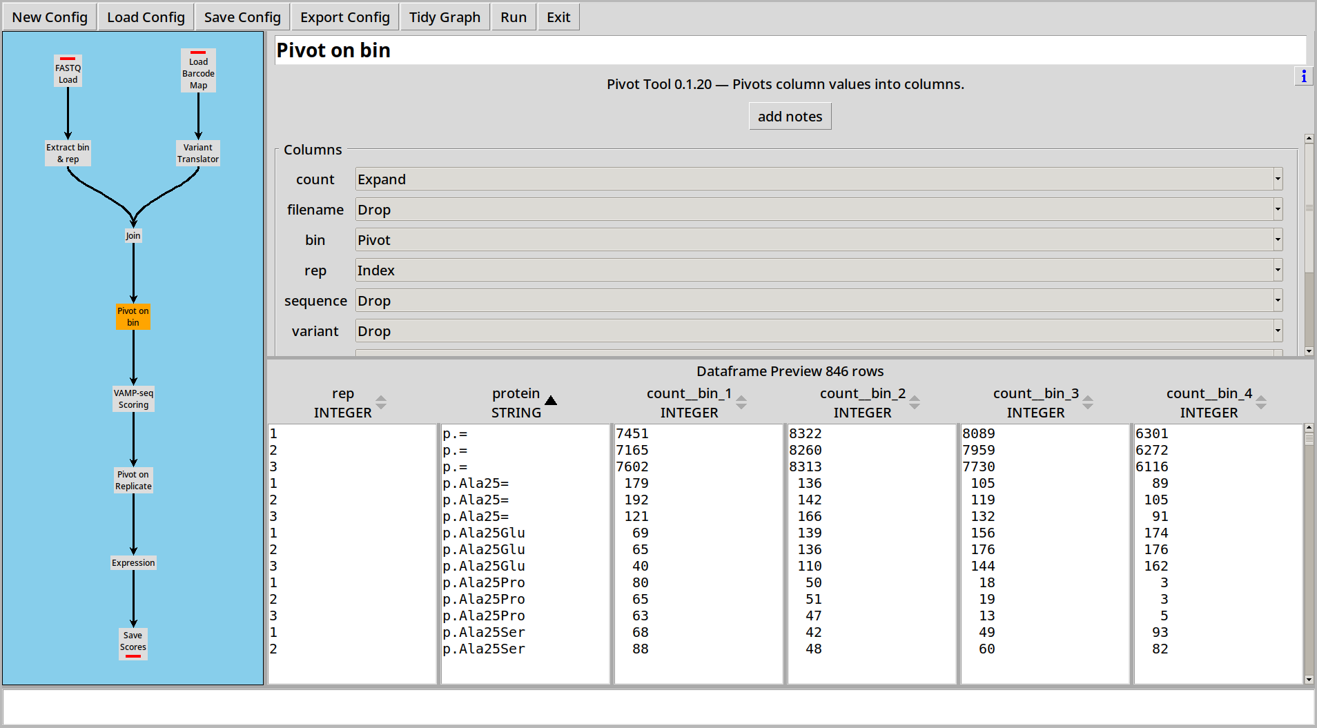
Then we can use the VAMPseq Plugin to calculate scores for each variant:

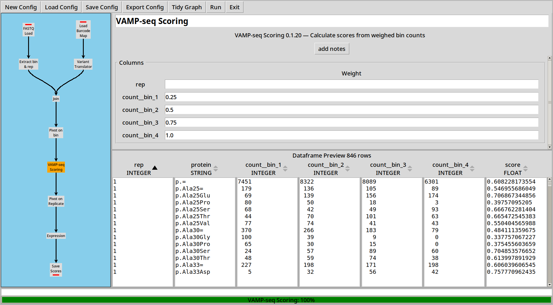
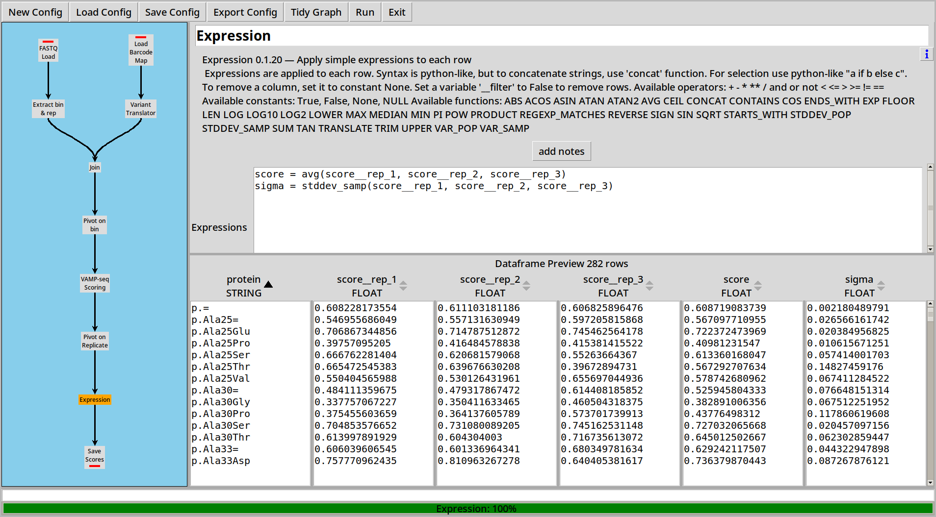
Combining Replicates

Once that’s done, pivot on replicate and use a simple formula to combine scores into an average score and an estimated standard deviation: